Reference: Denoising Diffusion Probabilistic Models, Ho et al., 2020

Introduction

Diffusion models are a powerful class of generative models that operate by systematically transforming data through two main processes: the forward process, where noise is gradually added to the data, and the reverse process, where this noise is removed to reconstruct the original data. These complementary steps allow the model to learn how to generate new data by working backward from noise.

At a high level:

• The forward process introduces noise to the data in small increments, progressively degrading its structure. This structured addition of noise creates a clear starting point for the reverse process.
• The reverse process learns to reconstruct the original data by iteratively removing noise, effectively reversing the steps of the forward process.

These processes are carefully designed using mathematical principles, such as Gaussian distributions, which model the noise, and Markov chains, which describe the step-by-step transitions. While these foundations are most prominent in Denoising Diffusion Probabilistic Models (DDPMs), they have inspired numerous advancements in the field, including non-Markovian approaches and models that operate in compressed latent spaces.

In this article, we focus on Denoising Diffusion Probabilistic Models (DDPMs) as they represent the foundational framework for diffusion models, introducing the mathematical principles and iterative processes that underpin this family of generative models. By understanding DDPMs, we can better appreciate how these principles extend to more advanced variants, such as Denoising Diffusion Implicit Models (DDIMs) and Latent Diffusion Models (LDMs), which address specific limitations of the original framework.

This article offers a high-level introduction to diffusion models, focusing on their core concepts and processes. While it simplifies some of the underlying mathematics, it provides a solid foundation for understanding DDPMs and their role in generative modeling. For readers seeking a deeper mathematical exploration, I recommend referring to the original paper by Ho et al. (2020).

In the sections ahead, we’ll explore the forward and reverse processes in detail, uncovering the mathematical framework behind their design and how these principles enable diffusion models to achieve remarkable results in generative AI tasks.

The Forward Diffusion Process: Breaking Down Data with Noise

The forward diffusion process is fundamental to diffusion models. Its purpose is to systematically add noise to data across multiple steps, gradually transforming it until it becomes indistinguishable from pure Gaussian noise. While this may initially seem like a destructive operation, it plays a critical role in setting up the reverse process, where the model will reconstruct the data step-by-step. By carefully controlling how noise is added, the forward process creates a structured pathway for the reverse process to follow, enabling precise reconstructions.

How the Forward Process Works

The forward diffusion process is mathematically described as a Markov chain. In a Markov chain, the state of the system at any given step depends only on the state of the previous step. This property simplifies the modeling and allows us to describe how noise is progressively introduced into the data.

At each time step \( t \), the data \( x \) transitions from \( x_{t-1} \) to \( x_t \) by adding a controlled amount of noise. This is expressed as:

\[ q(x_t | x_{t-1}) = \mathcal{N}(x_t; \sqrt{1-\beta_t} x_{t-1}, \beta_t I) \]

Here:

• \( x_t \): The noisy image (or data) at time step \( t \).
• \( x_{t-1} \): The image (or data) at the previous time step.
• \( \beta_t \): A small, time-dependent parameter that determines the amount of noise added at each step.
• \( \mathcal{N} \): A Gaussian distribution with mean \( \sqrt{1-\beta_t} x_{t-1} \) and variance \( \beta_t I \).
• \( I \): The identity matrix, which ensures that the noise added at each step is isotropic (uniform in all directions) and uncorrelated across dimensions.

This formulation shows how the forward process gradually transitions the data from its original structure to pure noise. Importantly, the process retains enough information in early steps for the model to later reconstruct the data during the reverse process.

Step-by-Step Noise Addition

The noise addition process can also be expressed in an equivalent form that highlights how \( x_t \) is computed directly from \( x_{t-1} \):

\[ x_t = \sqrt{1-\beta_t} x_{t-1} + \sqrt{\beta_t} \epsilon, \quad \epsilon \sim \mathcal{N}(0, I) \]

This equation ensures that \( x_t \) is a weighted combination of the previous state \( x_{t-1} \) and a Gaussian noise component \( \epsilon \), where:

1. The term \( \sqrt{1-\beta_t} x_{t-1} \) retains a proportion of the original data’s structure, scaled by \( \sqrt{1-\beta_t} \).
2. The term \( \sqrt{\beta_t} \epsilon \) introduces random noise, scaled by \( \sqrt{\beta_t} \), which gradually degrades the data.

By balancing these two components, the forward process transforms the data into progressively noisier states. The added noise follows a carefully designed schedule, preserving meaningful information during the early steps while gradually transitioning the data to a Gaussian distribution in the later steps. Additionally, the use of Gaussian noise aligns naturally with the assumptions of the Markov chain, ensuring that each state \( x_t \) remains a Gaussian distribution.

The Role of the Noise Scheduler

The parameter \( \beta_t \), which controls the amount of noise added at each step, is part of a pre-defined noise schedule. This schedule is typically designed by engineers to balance two competing goals:

• In the early steps: Smaller \( \beta_t \) values ensure that much of the original structure is retained, providing the reverse process with sufficient information for reconstruction.
• In the later steps: Larger \( \beta_t \) values accelerate the degradation into pure noise, ensuring the final state is a standard Gaussian distribution.

Commonly used schedules include linear or quadratic increases in \( \beta_t \) over time, though custom schedules can be designed for specific applications. The choice of schedule is critical, as it determines the quality and efficiency of the model during both the forward and reverse processes.

Why Add Noise?

Although the forward process might appear to be simply degrading the data, it is essential for the training and functionality of diffusion models. By systematically corrupting the data with noise, the forward process provides the model with a structured learning objective: learn to reverse this process by predicting and removing the added noise. The gradual introduction of noise also allows the model to learn relationships between different levels of data corruption, making the reverse process both feasible and effective.

In essence, the forward process lays the groundwork for the reverse process, carefully preserving enough information in each step to enable the model to reconstruct the original data with high precision. This structured degradation serves as a blueprint for generative tasks, allowing the model to produce high-quality data reconstructions from noise.

The Reverse Diffusion Process: Reconstructing Data from Noise

Reference: Denoising Diffusion Probabilistic Models, Ho et al., 2020

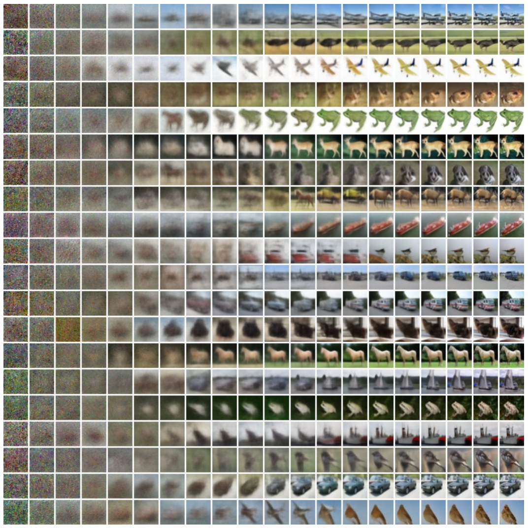
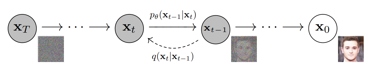
While the forward process systematically adds noise to transform data into random Gaussian noise, the reverse process does the opposite. It removes the noise step-by-step, progressively reconstructing the original data. This reconstruction relies on a learned model that predicts the noise added during the forward process. By leveraging the structure introduced by the forward process, the reverse process enables high-quality reconstructions. Let’s explore the mechanics in detail.

Theoretical Basis of the Reverse Process

The reverse process is theoretically derived using Bayes’ rule, which establishes the relationship between the forward and reverse transitions. Specifically, Bayes’ rule expresses the reverse transition \( p_\theta(x_{t-1} | x_t) \) as:

\[ p_\theta(x_{t-1} | x_t) \propto q(x_t | x_{t-1}) \cdot p_\theta(x_{t-1}) \]

Here:

• \( q(x_t | x_{t-1}) \): The forward noise distribution, a Gaussian distribution defined during the forward process.
• \( p_\theta(x_{t-1}) \): The prior over the data, often assumed to be Gaussian as well.

This relationship highlights that the reverse process is mathematically dependent on the forward process. The structure introduced by the forward process provides a blueprint for reconstruction. However, in practice, the reverse process avoids directly computing this product. Instead of directly computing this product, a neural network predicts the noise added during the forward process, simplifying the problem and ensuring computational efficiency.

To achieve this, the reverse process is modeled as a Markov chain, where each step depends only on the current noisy state \( x_t \). The transition from \( x_t \) to \( x_{t-1} \) is expressed as:

\[ p_\theta(x_{t-1} | x_t) = \mathcal{N}(x_{t-1}; \mu_\theta(x_t, t), \Sigma_\theta(x_t, t)) \]

This represents a Gaussian distribution with:

• Mean \( \mu_\theta(x_t, t) \): A learned function that predicts the most likely denoised version of \( x_t \) at each step.
• Variance \( \Sigma_\theta(x_t, t) \): The uncertainty in the prediction. This is often fixed for simplicity but can also be learned by the model.

The learned mean and variance allow the reverse process to iteratively refine the noisy data, gradually removing the noise until the original data is reconstructed.

Predicting Noise Instead of Data

Instead of directly predicting \( x_{t-1} \), the reverse process focuses on predicting the noise \( \epsilon \) added during the forward process. A neural network, denoted as \( \epsilon_\theta(x_t, t) \), is trained to learn this mapping. Predicting noise rather than \( x_{t-1} \) offers two key advantages:

• Simpler training: Noise follows a standard Gaussian distribution, making it easier to model compared to the complex data distribution of \( x_{t-1} \).
• Reconstruction through noise: Once the noise \( \epsilon \) is predicted, it can be used to compute \( x_{t-1} \) directly using the following equation:

\[ x_{t-1} = \frac{1}{\sqrt{1-\beta_t}} \left( x_t - \sqrt{\beta_t} \epsilon_\theta(x_t, t) \right) + \sigma_t z \]

This equation is derived from the Gaussian distribution used to model the reverse transition, introduced in the previous section.

Here:

• \( \sqrt{1-\beta_t} \): A scaling factor that retains the contribution of the signal from \( x_t \).
• \( \sqrt{\beta_t} \epsilon_\theta(x_t, t) \): The predicted noise contribution, subtracted from \( x_t \).
• \( \sigma_t z \): Optional Gaussian noise (\( z \sim \mathcal{N}(0, I) \)), introduced to maintain stochasticity during reconstruction.

This formulation allows the reverse process to iteratively refine the data step-by-step, gradually removing the noise until \( x_0 \), the original data, is reconstructed.

Training the Reverse Process

At the core of diffusion models is the ability to accurately predict the noise added during the forward process. Training the reverse process involves teaching a neural network, \( \epsilon_\theta(x_t, t) \), to predict this noise \( \epsilon \) at each timestep \( t \). This learned mapping is critical for reconstructing data during inference, as it enables the model to progressively reverse the diffusion process.

The training begins with data samples \( x_0 \), the original data points from the target distribution. These samples are progressively noised through the forward diffusion process, generating a series of intermediate states \( x_1, x_2, \dots, x_T \), where \( T \) is the final timestep. At each timestep \( t \), a noisy sample \( x_t \) is produced using the equation:

\[ q(x_t | x_{t-1}) = \mathcal{N}(x_t; \sqrt{1-\beta_t} x_{t-1}, \beta_t I). \]

To train the reverse process, we need to construct a supervised learning task. The ground truth for this task is the noise \( \epsilon \) that was added to produce \( x_t \) from \( x_{t-1} \). The neural network \( \epsilon_\theta(x_t, t) \) is trained to minimize the difference between the true noise \( \epsilon \) and the noise predicted by the model. This is achieved using the following objective function:

\[ \mathcal{L}_{\text{simple}} = \mathbb{E}_{x_0, \epsilon, t} \left[ \| \epsilon - \epsilon_\theta(x_t, t) \|^2 \right]. \]

Here:

• \( x_0 \): The original data sample.
• \( \epsilon \): The Gaussian noise added during the forward process to create \( x_t \) from \( x_{t-1} \), sampled as \( \epsilon \sim \mathcal{N}(0, I) \).
• \( t \): The timestep, which is input into the neural network alongside \( x_t \) to indicate the current step of the reverse process.
• \( x_t \): The noisy data at timestep \( t \), generated using the forward process.

To calculate \( \epsilon \), we start by generating the noisy sample \( x_t \) directly from \( x_0 \) using the forward process:

\[ x_t = \sqrt{\bar{\alpha}_t} x_0 + \sqrt{1 - \bar{\alpha}_t} \epsilon, \]

where \( \bar{\alpha}_t = \prod_{i=1}^t (1 - \beta_i) \) is the cumulative product of the noise schedule. Rearranging this equation, \( \epsilon \) can be isolated as:

\[ \epsilon = \frac{x_t - \sqrt{\bar{\alpha}_t} x_0}{\sqrt{1 - \bar{\alpha}_t}}. \]

This definition of \( \epsilon \) explicitly connects the noisy sample \( x_t \) and the original data \( x_0 \). It is directly used as the ground truth for the loss function, \( \mathcal{L}_{\text{simple}} \), which trains the noise prediction network \( \epsilon_\theta(x_t, t) \). In this way, the forward process provides the foundation for constructing the supervised learning task that enables the reverse process to reconstruct clean data during inference.

During training, the model learns to predict the noise \( \epsilon \), which is essential for reconstructing data during inference. By accurately predicting \( \epsilon \), the model becomes capable of progressively reversing the forward diffusion process, starting from \( x_T \), which is pure Gaussian noise, and iteratively denoising until it recovers \( x_0 \).

In inference, the reverse process uses the predicted noise \( \epsilon_\theta(x_t, t) \) at each timestep \( t \) to iteratively denoise \( x_t \). This is achieved using the equation:

\[ x_{t-1} = \frac{1}{\sqrt{1-\beta_t}} \left( x_t - \sqrt{\beta_t} \epsilon_\theta(x_t, t) \right) + \sigma_t z, \]

where \( z \sim \mathcal{N}(0, I) \) optionally introduces stochasticity, allowing for diverse outputs.

The reverse process leverages the Gaussian structure of the forward diffusion process. During training, the model learns the relationship between noisy data \( x_t \) and the added noise \( \epsilon \), guided by the forward process distribution \( q(x_t | x_{t-1}) \). In inference, this mapping is applied iteratively using the same noise schedule \( \beta_t \) from training to systematically remove noise.

By aligning the forward and reverse processes, the model accurately predicts noise and reconstructs high-quality data from pure noise. Training a diffusion model is essentially about training a noise prediction network, enabling the model to understand the relationship between noisy and clean data across all levels of corruption. This iterative process allows the model to reverse the forward diffusion process step-by-step, producing high-quality outputs from noise with remarkable precision, making diffusion models excel in generative tasks.

Output Control in DDPMs

In their basic form, diffusion models lack explicit mechanisms to control the specific outputs they generate. This is because the reverse process starts from pure Gaussian noise \( x_T \), which contains no signal, requiring the noise prediction model \( \epsilon_\theta(x_t, t) \) to iteratively reconstruct data from this randomness. Since the initial sample \( x_T \) is entirely random, the outputs of the model are inherently stochastic and unpredictable. At this stage, no meaningful structure is present, making it challenging to guide the generation process toward specific outcomes.

However, various techniques have been developed to introduce control into diffusion models. One common approach is conditioning, where additional information, such as text descriptions, class labels, or specific latent encodings, guides the reverse process toward desired outputs. Latent Diffusion Models (LDMs), including Stable Diffusion, further enhance control by operating in a compressed latent space rather than the original data space. By learning a lower-dimensional representation of the data, LDMs significantly reduce computational requirements while maintaining high-quality generation. This efficiency makes them well-suited for large-scale applications, such as text-to-image synthesis, where textual prompts provide precise control over generated outputs.

As of January 2025, latent diffusion remains one of the most effective techniques for high-resolution image synthesis, striking a balance between efficiency and output fidelity. Other approaches, such as classifier guidance or score-based conditioning, offer additional ways to refine and control outputs, though each comes with trade-offs depending on the specific application.

Challenges and Practical Limitations

Denoising Diffusion Probabilistic Models (DDPMs) introduced a powerful framework for generative modeling, but their design also comes with notable challenges and limitations. A primary concern is the computational cost associated with both training and inference. The reverse process in DDPMs requires hundreds or even thousands of iterative denoising steps, with each step involving a forward pass through the model. This makes inference significantly slower compared to other generative methods like GANs, which generate outputs in a single pass. Additionally, training DDPMs demands substantial computational resources, as large datasets must be processed over many iterations, posing a barrier for smaller organizations or developers with limited hardware.

Another challenge lies in the dependence on carefully designed noise schedules \( \beta_t \). These schedules control how noise is added during the forward process and removed during the reverse process. Poorly chosen schedules can destabilize training or degrade the quality of generated outputs, requiring extensive experimentation to optimize. This reliance on tuning noise schedules makes DDPMs less practical for certain real-world applications where efficiency is a priority.

Scaling diffusion models to high-resolution data introduces additional difficulties. As the resolution increases, so do memory and computational requirements, which grow exponentially. Even advanced variants like Stable Diffusion, which operate more efficiently, face constraints when working with extremely high-resolution outputs or computationally intensive applications.

Diffusion models also face challenges in achieving consistent control over their outputs. While conditioning techniques, such as using text descriptions, class labels, or latent representations, have improved control, achieving consistent, reproducible results remains difficult, particularly for complex or multimodal datasets. Fine-tuning pre-trained diffusion models for specific domains adds another layer of complexity. As of January 2025, fine-tuning remains computationally expensive, limiting accessibility for smaller organizations or individuals. However, advances such as Low-Rank Adaptation (LoRA) and other parameter-efficient fine-tuning methods offer promising solutions to make this process more efficient and accessible in the near future.

Despite these limitations, the evolution of diffusion models has addressed many of the shortcomings of DDPMs. For example, Denoising Diffusion Implicit Models (DDIMs) introduced a non-Markovian framework that significantly accelerates inference by reducing the number of required steps while maintaining high-quality outputs. Similarly, Latent Diffusion Models (LDMs) transformed diffusion modeling by operating in a compressed latent space instead of the original data space, reducing memory and computational costs while enabling high-resolution generation.

These innovations have paved the way for models like Stable Diffusion, which exemplify how latent diffusion techniques can balance computational efficiency with impressive control over outputs. While Stable Diffusion has been a landmark development, the field of diffusion models is evolving rapidly. Emerging techniques continue to push the boundaries of generative modeling, exploring faster inference, improved scalability, and greater flexibility across diverse applications. Diffusion models are far from reaching their full potential, and the future promises even more exciting advancements in this dynamic area of AI research.

Conclusion

This article provided an accessible overview of the mathematical foundations of diffusion models, focusing on the forward and reverse processes that enable their remarkable generative capabilities. By introducing concepts like Gaussian distributions, Markov chains, and the systematic addition and removal of noise, we’ve explored how Denoising Diffusion Probabilistic Models (DDPMs) lay the groundwork for this powerful class of generative models.

While DDPMs serve as a foundational framework, advancements such as Denoising Diffusion Implicit Models (DDIMs) and Latent Diffusion Models (LDMs) have addressed key challenges like computational efficiency and scalability. These innovations highlight how mathematical insights continue to drive the evolution of diffusion models, transforming them into practical tools for real-world applications.

This article intentionally simplifies many of the mathematical details to make the concepts more accessible. For readers interested in a deeper exploration, including rigorous derivations and empirical benchmarks, I encourage consulting the original DDPM paper by Ho et al. (2020).